Image Mosaics and Panorama Stitching

github.com/aditimundra05/cs180/4/index.html

Part A.1: Shoot the Pictures

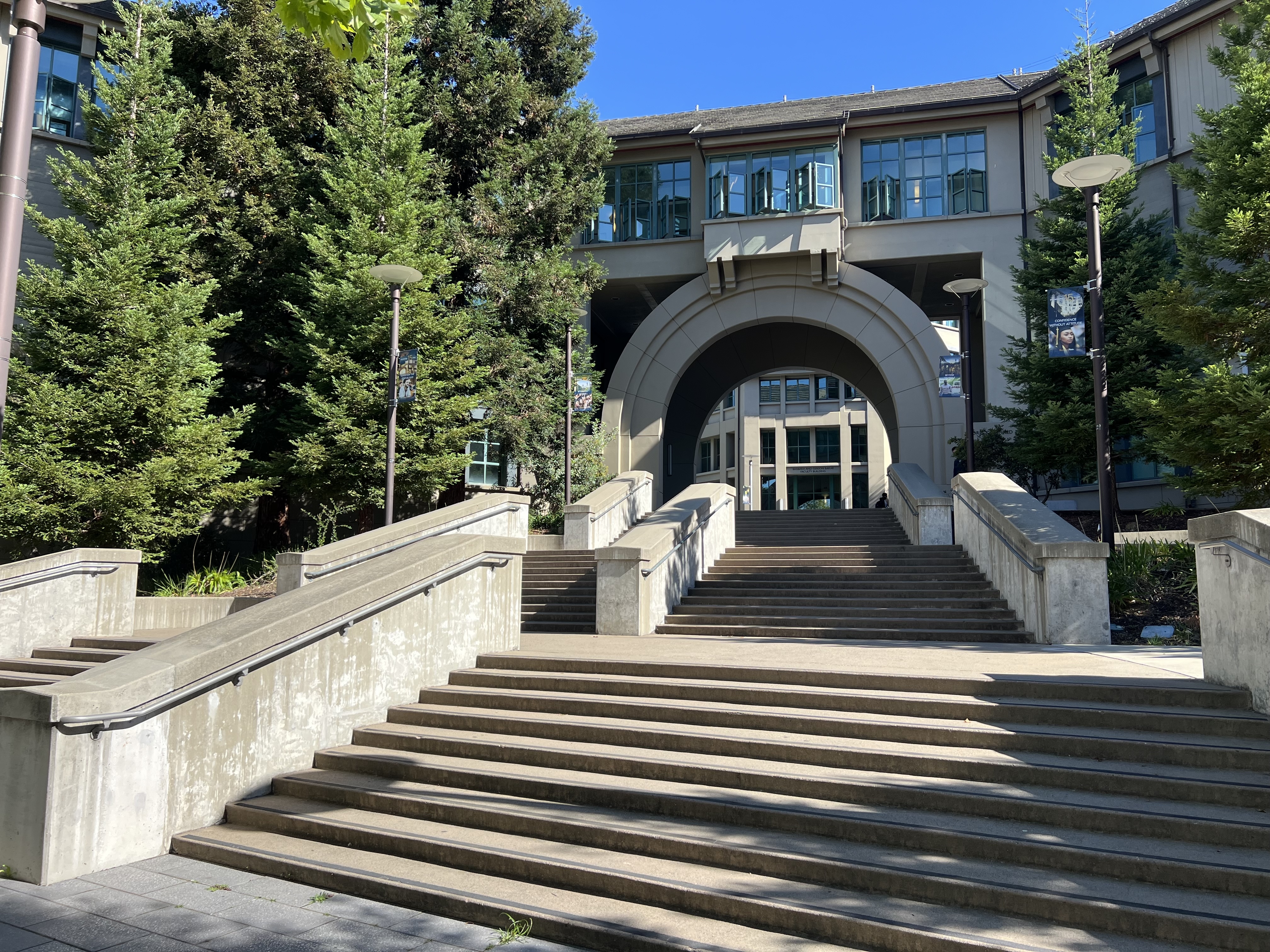
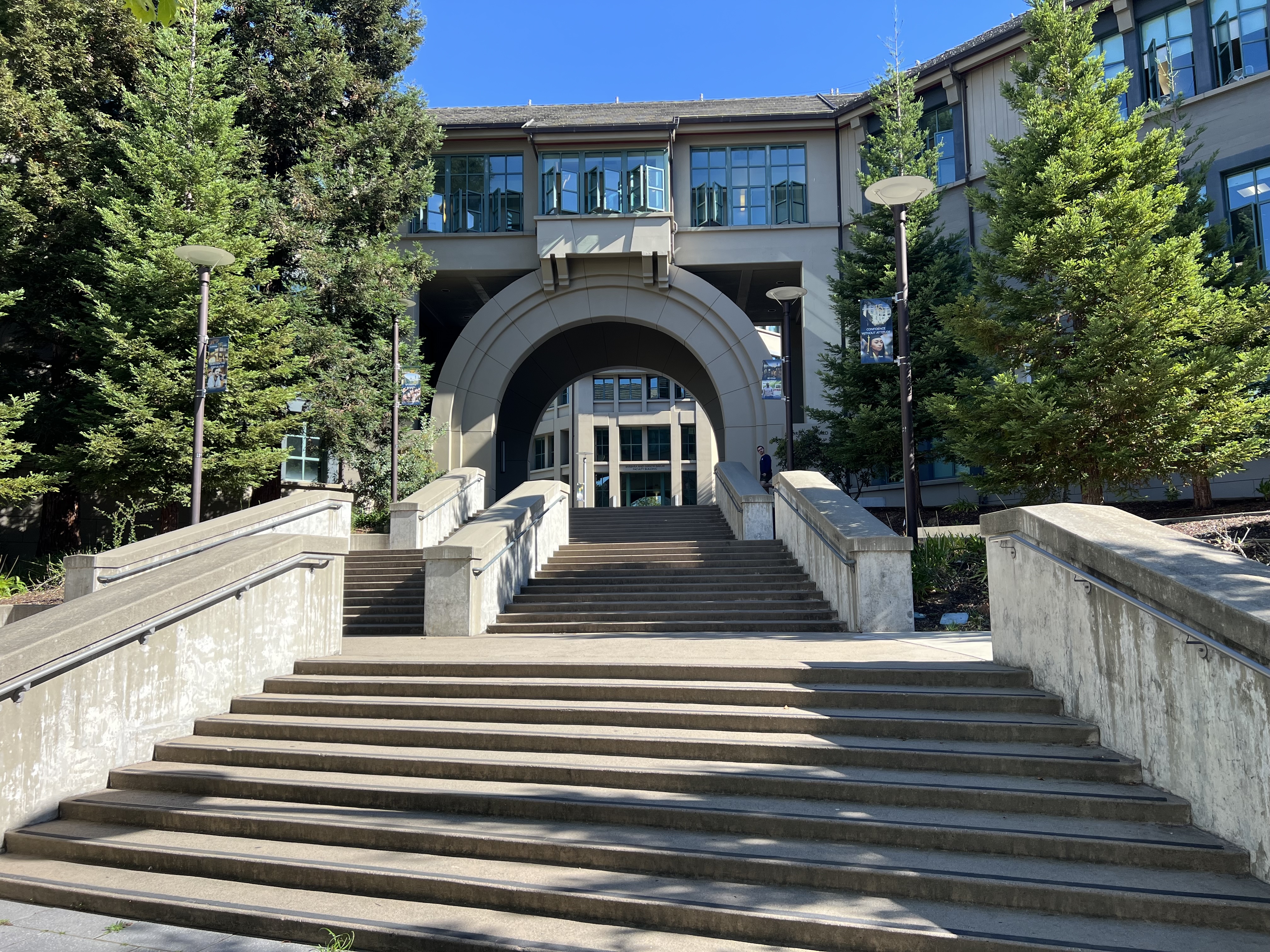
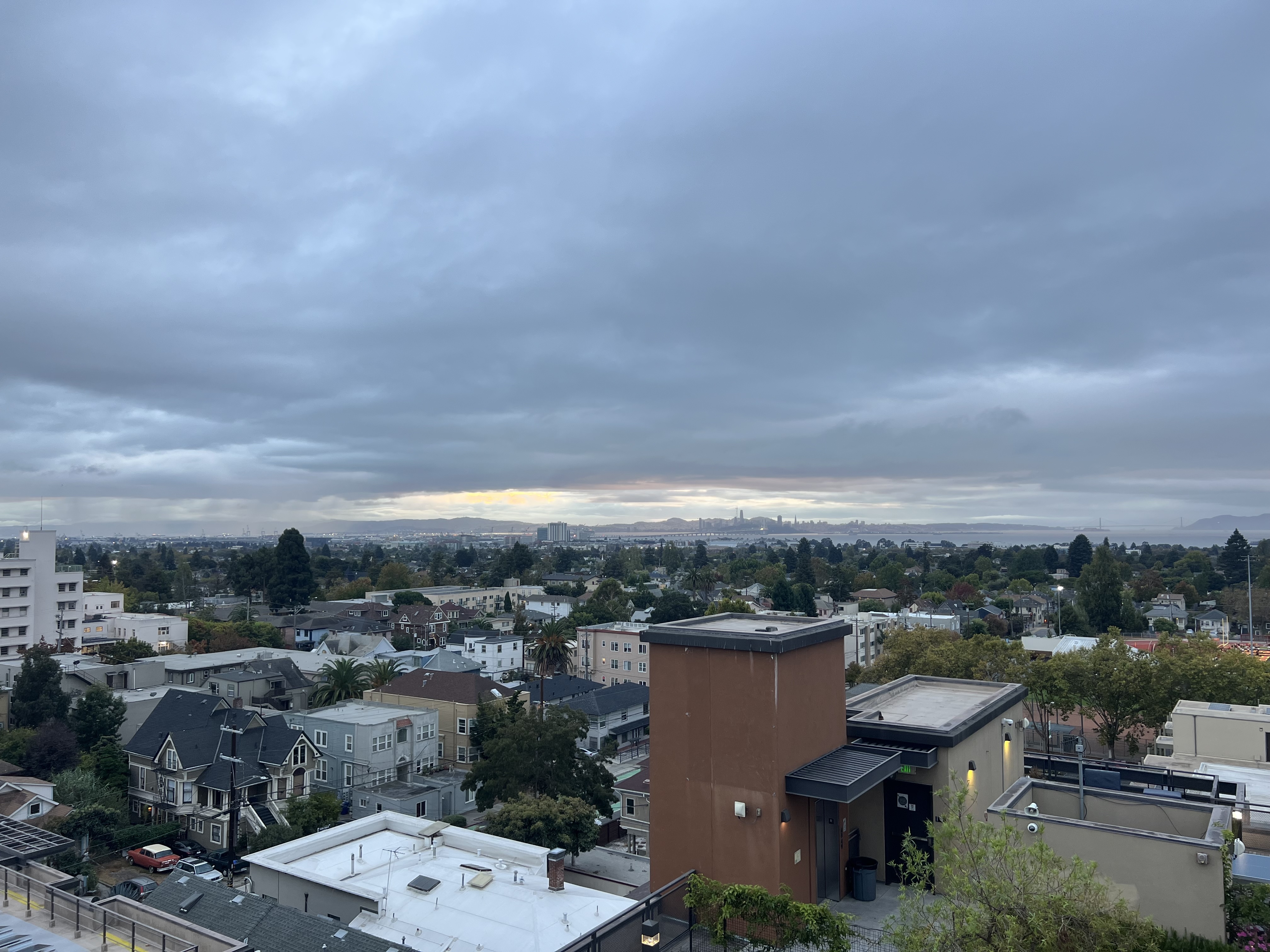
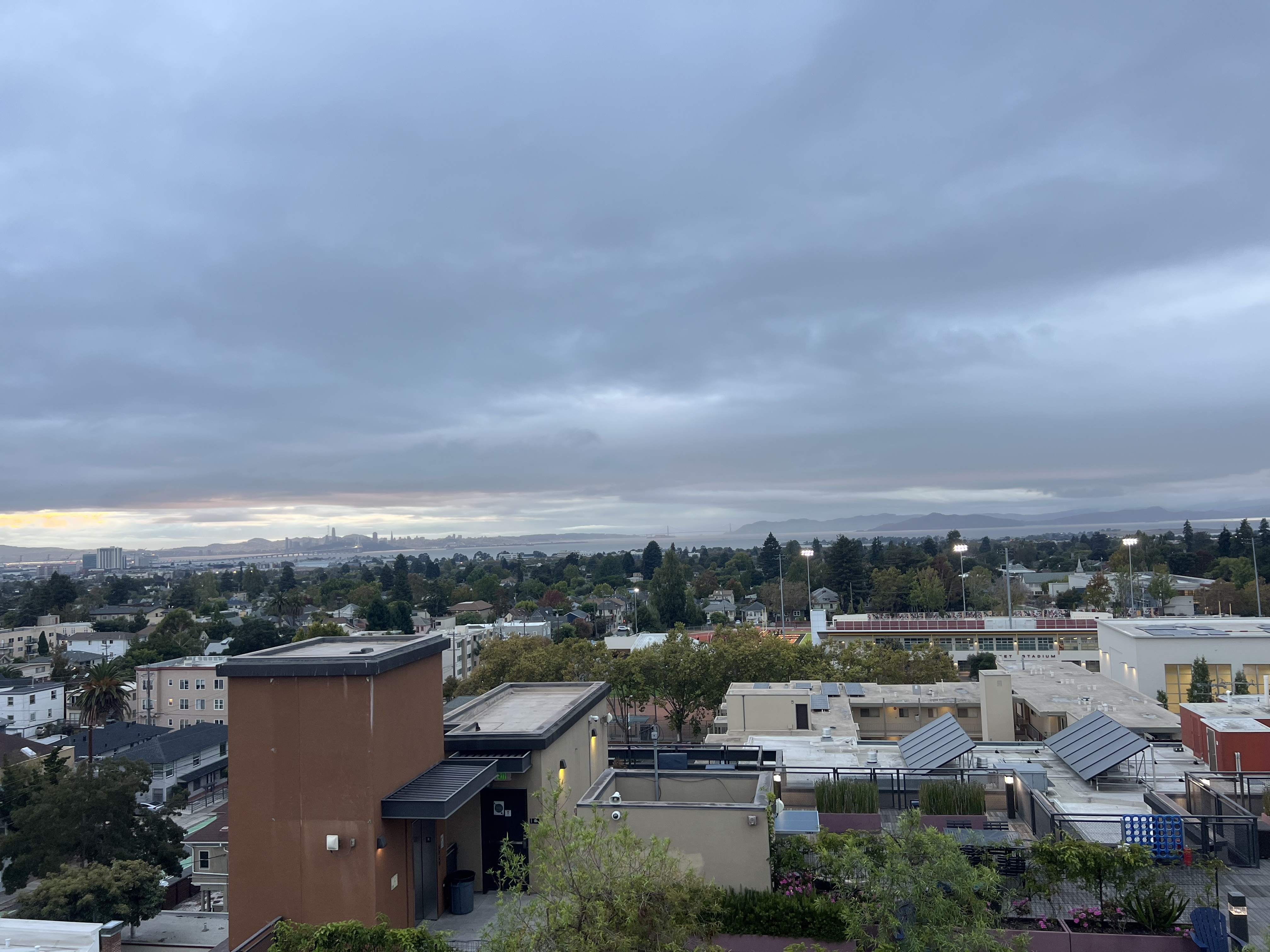
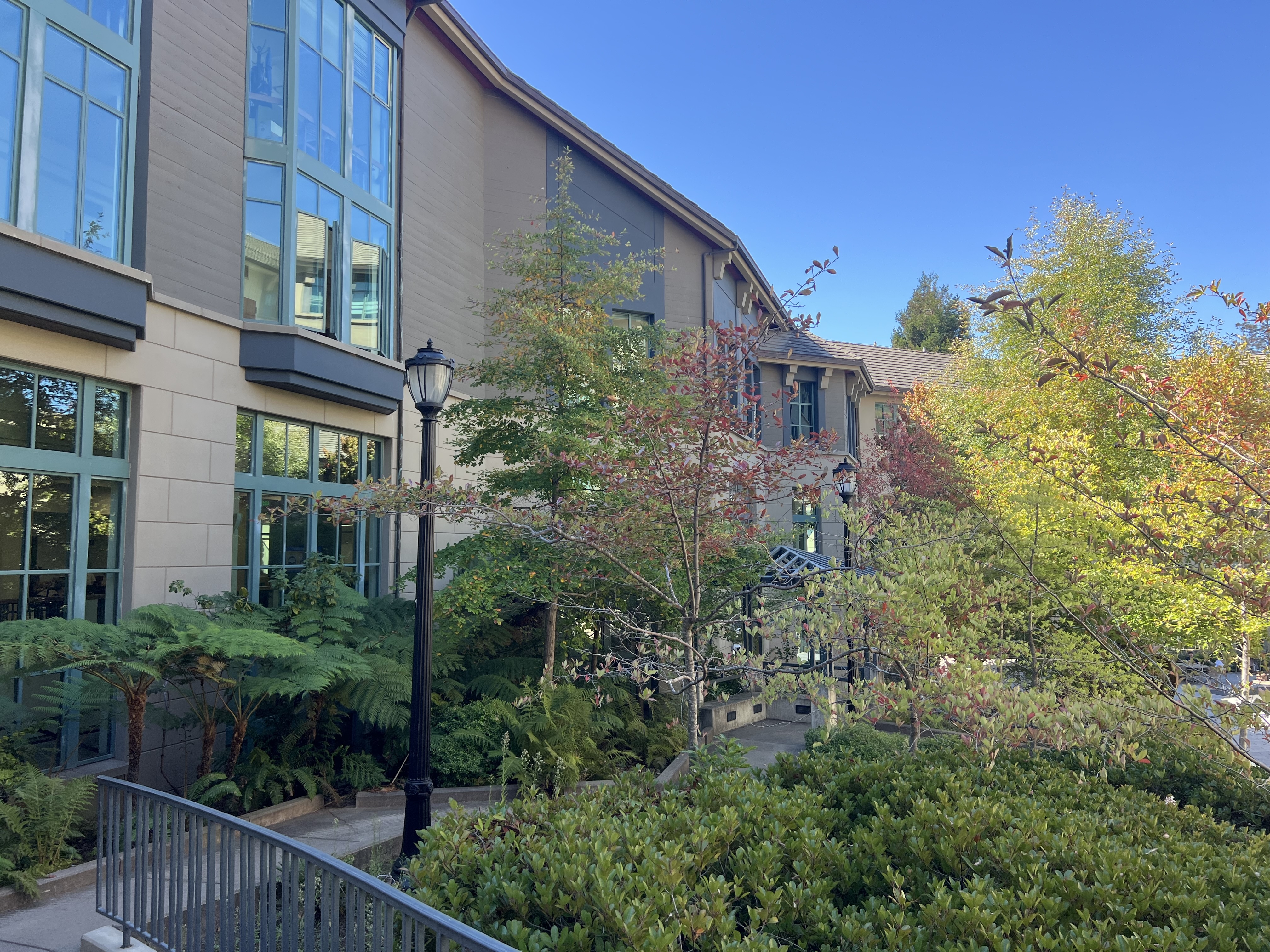
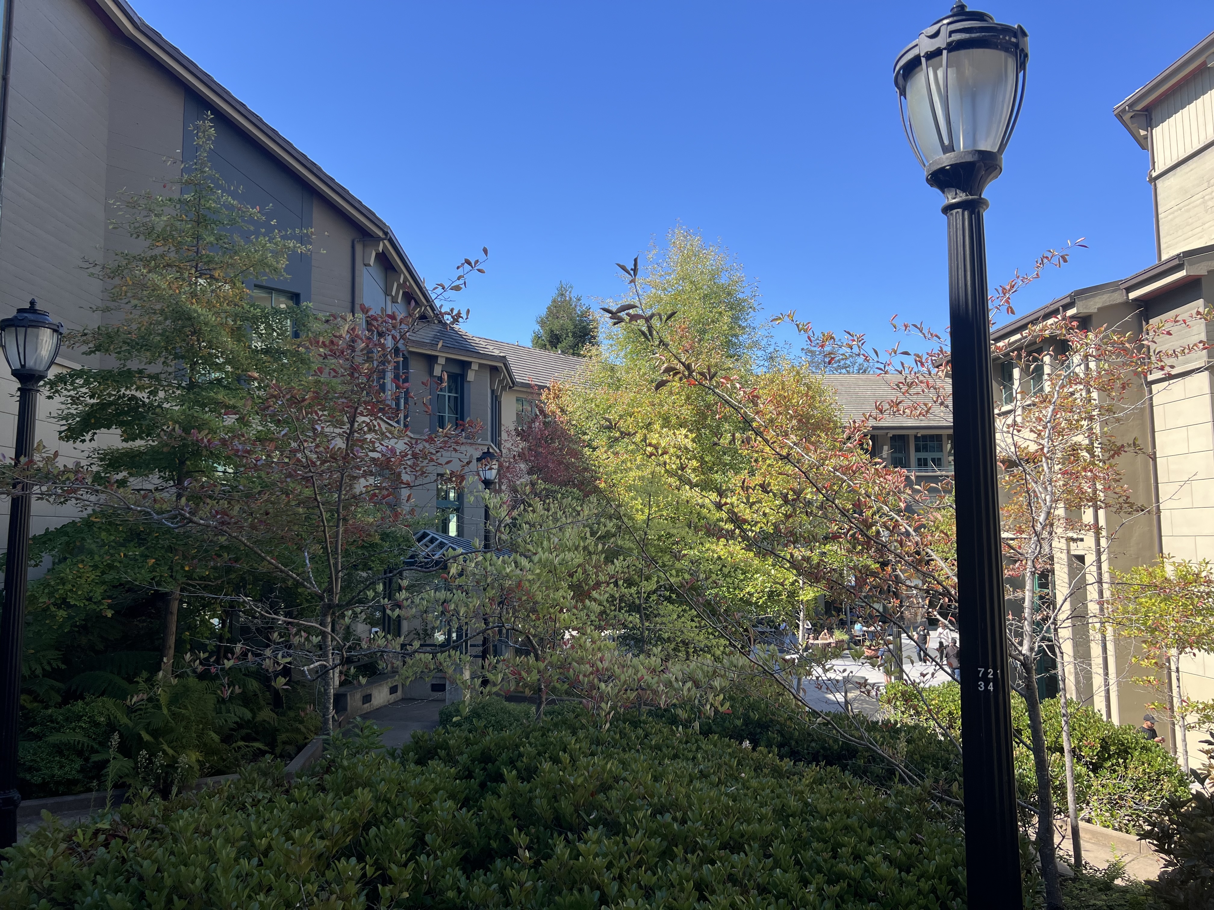
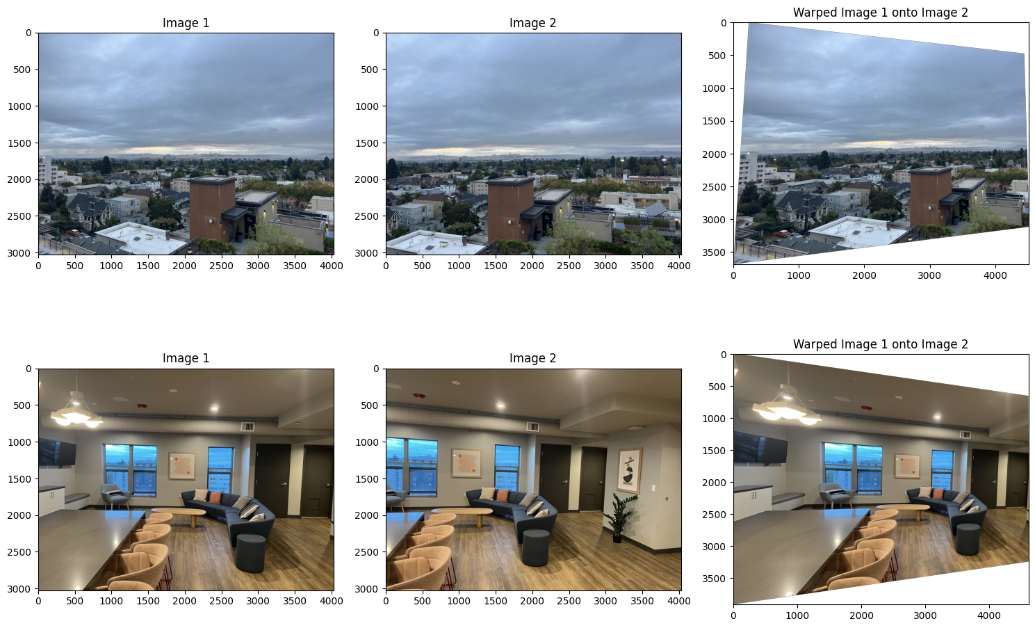
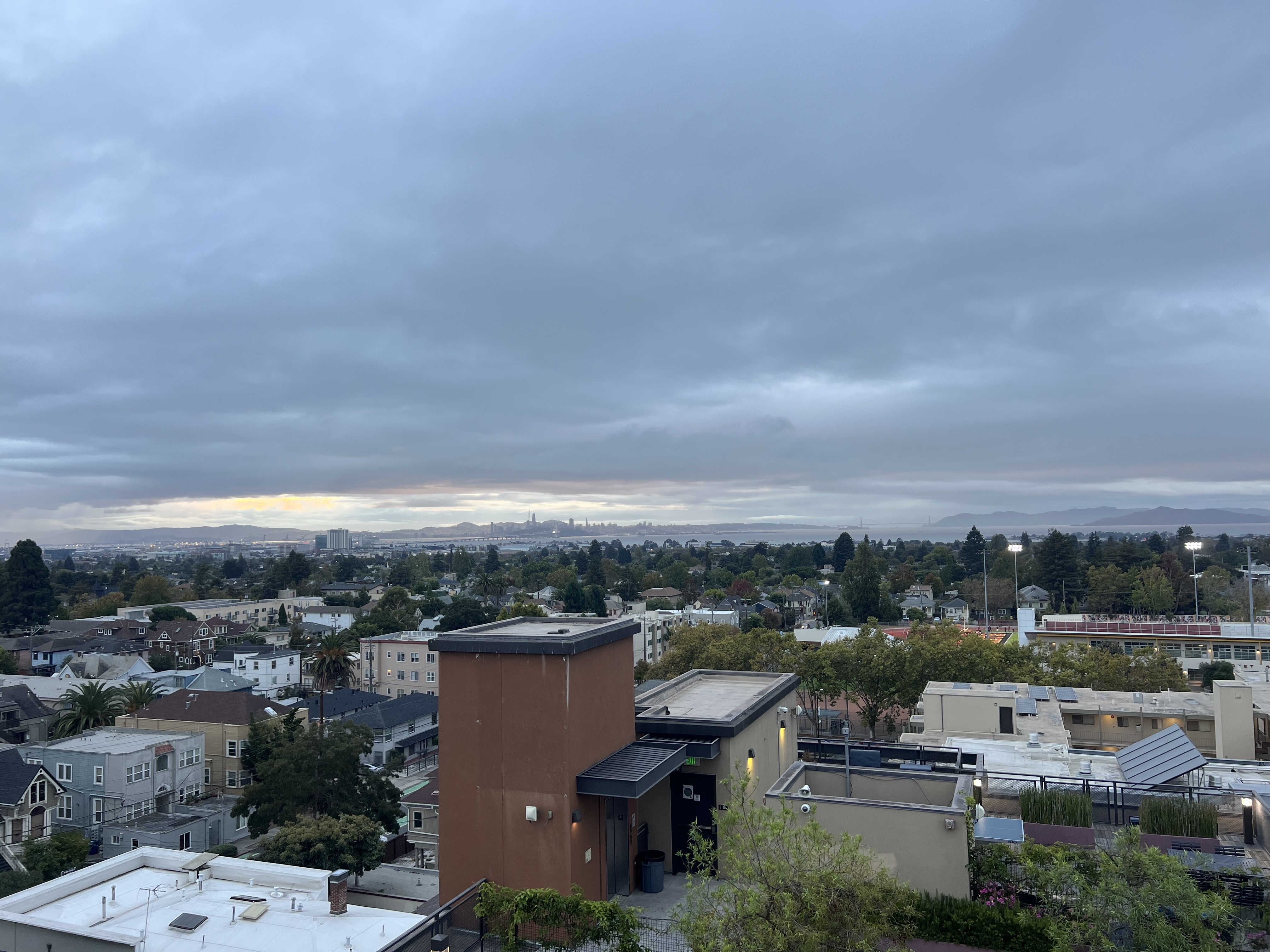
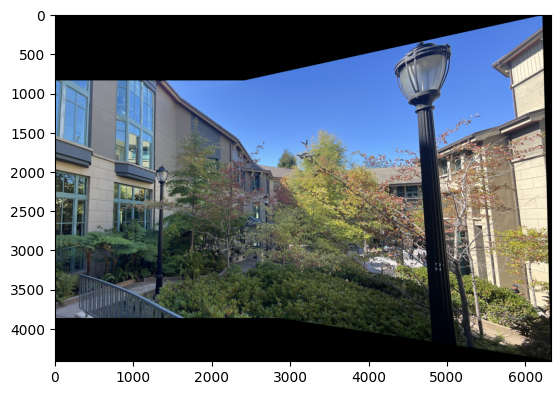
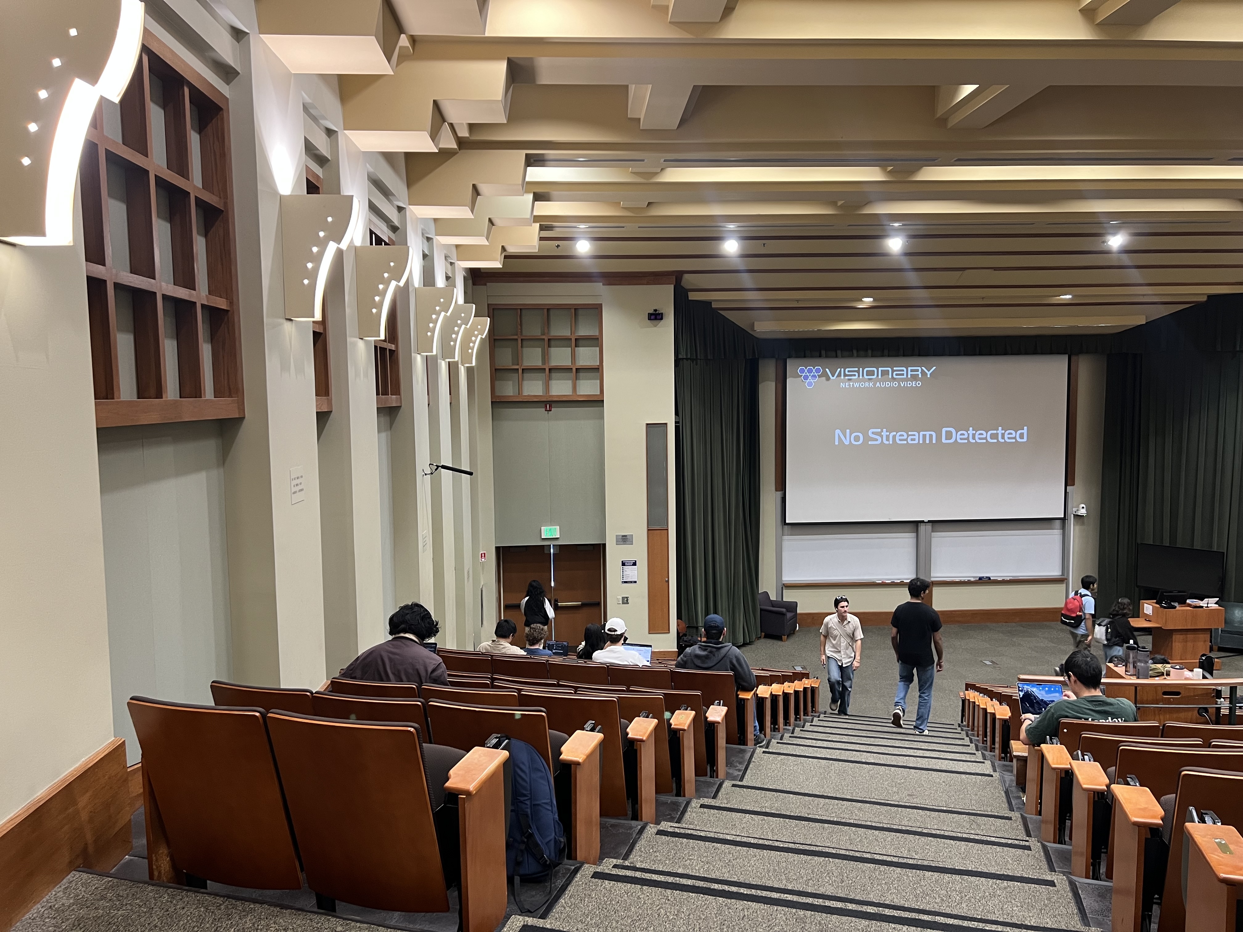
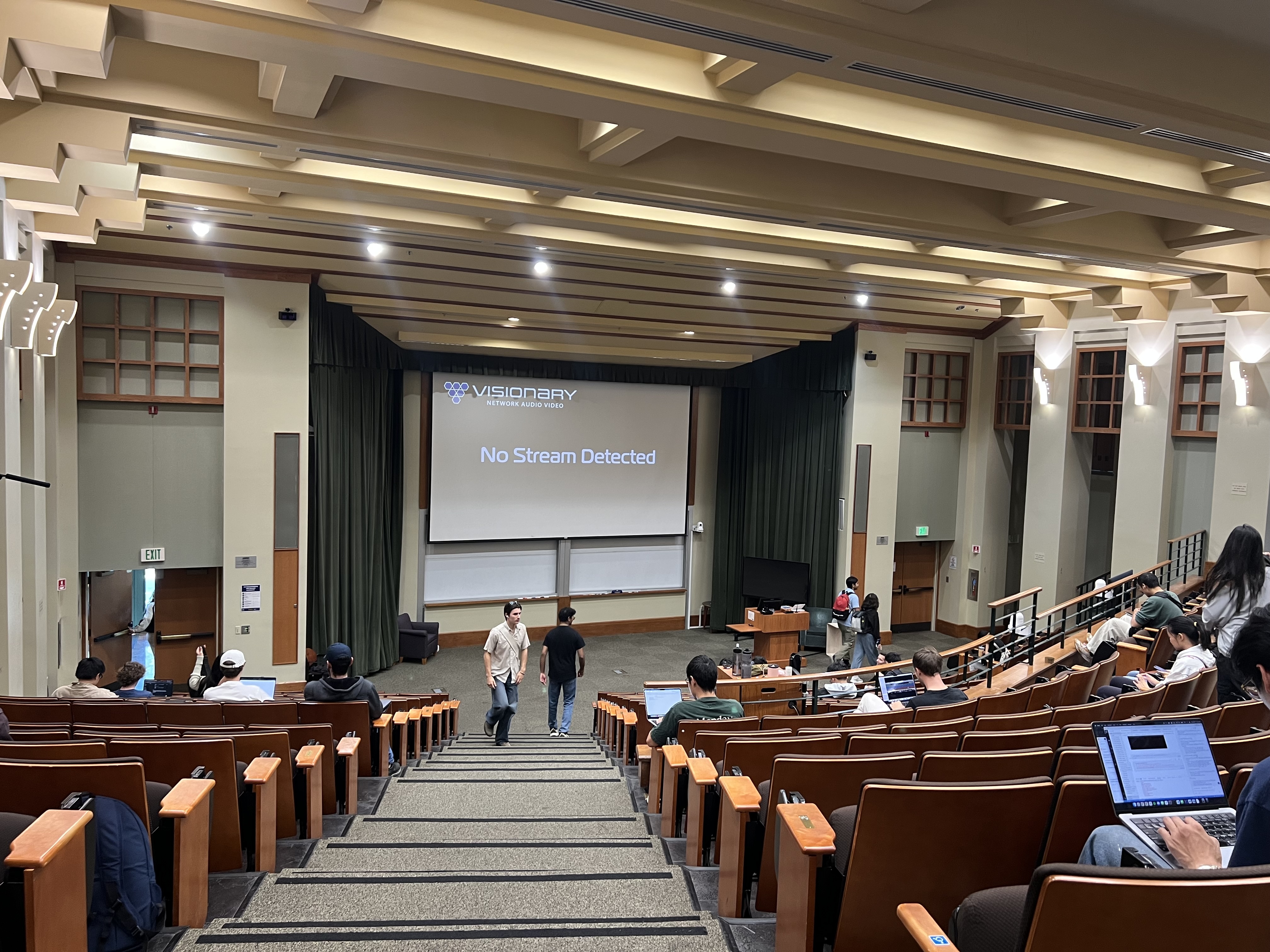
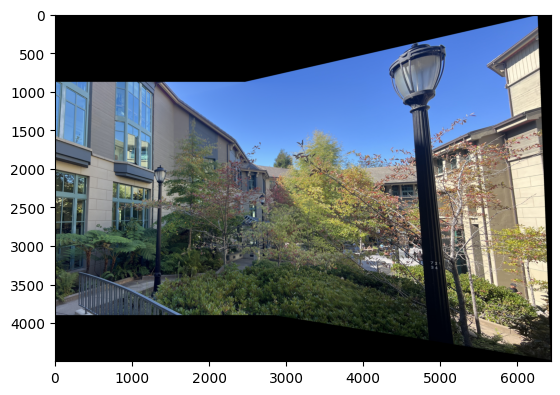
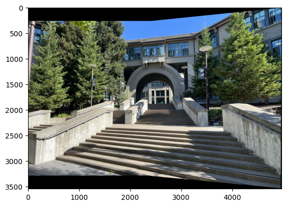
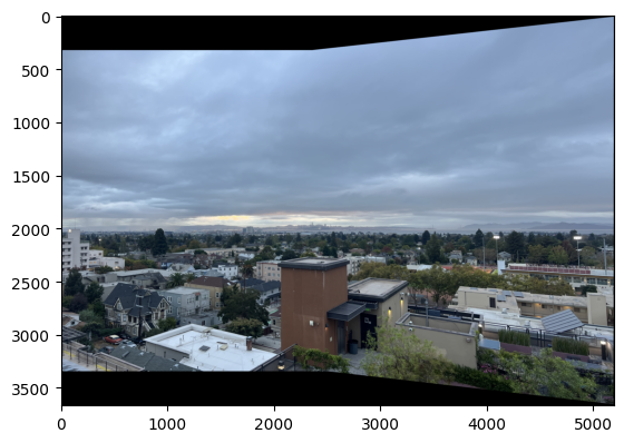
In order to create panoramic mosaics, I took pictures of the Haas Faculty building, the rooftop of my apartment, and outside the library. I fixed the center of projection and rotated my camera while capturing the photos, kept 40% of overlap between the images, and shot in a short time span.

Image Set 1: Haas Faculty Arch

Haas 1

Haas 2

Image Set 2: Berkeley Landscape

Landscape 1

Landscape 2

Image Set 3: Library Trees

Library 1

Library 2

Part A.2: Recover Homographies

A homography is a projective transformation that maps points from one image plane to another. Mathematically, it relates corresponding points \( \mathbf{p} \) and \( \mathbf{p}' \) between two images as:

\mathbf{p}' = H\mathbf{p}

where \( H \) is a 3×3 matrix with 8 degrees of freedom (the lower-right element is set to 1 for normalization).

Procedure

First, I used the tool given to find point correspondences between the two images. Given corresponding points in homogeneous coordinates:

\mathbf{p} = \begin{bmatrix}x\\y\\1\end{bmatrix} \quad \mathbf{p}' = \begin{bmatrix}x'\\y'\\1\end{bmatrix}

and the homography matrix:

H = \begin{bmatrix}h_1&h_2&h_3\\ h_4&h_5&h_6 \\h_7&h_8&1\end{bmatrix}

The transformation yields:

H\mathbf{p} = \begin{bmatrix} xh_1+yh_2+h_3\\ xh_4+yh_5+h_6\\ xh_7+yh_8+1 \end{bmatrix}

Then, I normalized using the z component to come back to the original (x, y) plane, and obtained:

\begin{cases} \frac{xh_1+yh_2+h_3}{xh_7+yh_8+1} = x'\\ \\ \frac{xh_4+yh_5+h_6}{xh_7+yh_8+1} = y' \end{cases}

As per discussion, I learned that we can rearrange these equations to get two linear constraints per point correspondence:

\begin{bmatrix} x & y & 1 & 0 & 0 & 0 & -x'x & -x'y\\ 0 & 0 & 0 & x & y & 1 & -y'x & -y'y \end{bmatrix} \begin{bmatrix}h_1\\h_2\\h_3\\h_4\\h_5\\h_6\\h_7\\h_8\end{bmatrix} = \begin{bmatrix}x'\\ y'\end{bmatrix}

For \( n \) point correspondences, we construct an overdetermined system \( A\mathbf{h} = \mathbf{b} \) where \( A \) is a \( 2n \times 8 \) matrix, and solve using least squares: \( \mathbf{h} = (A^TA)^{-1}A^T\mathbf{b} \).

Point Correspondences

Here are my point correspondences for the images.

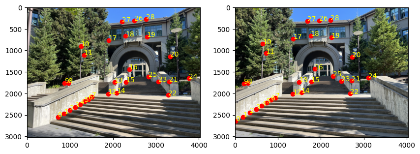
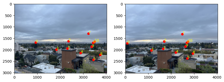
Visualized point correspondences between two images

Recovered Homography Matrix

Using the point correspondences shown above, the computed homography matrix is:

H_haas = [[ 1.30315558e+00  2.16205768e-03 -9.27599325e+02]
 [ 1.15292498e-01  1.17892236e+00 -2.81916782e+02]
 [ 7.32444026e-05  3.82886816e-06  1.00000000e+00]]

H_landscape = [[ 1.33437925e+00 -4.47218776e-02 -1.07262312e+03]
 [ 1.40441962e-01  1.13252177e+00 -2.39534564e+02]
 [ 9.44219893e-05 -2.51788604e-05  1.00000000e+00]]

Part A.3: Warp the Images

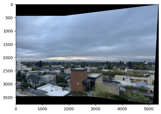
Once the homography is recovered, we can warp images to align them. I implemented two interpolation methods using inverse warping to avoid holes in the output:

Inverse Warping

Rather than mapping source pixels to destination (forward warping), which can leave holes since pixels can hit some of the same points during their transformation while leaving others untouched (essentially no pixels map to that place), I used inverse warping. For each pixel in the output image, I computed its corresponding location in the source image using \( H^{-1} \) and interpolated the color value. First, I found the location of the destination image by applying H to the corners of my source image. From this bounding box, I went coordinate by coordinate and applied H_inverse to find the source location. Here, I applied the respective interpolation methods detailed below.

Interpolation Methods

1. Nearest Neighbor Interpolation

In this method, I rounded the computed coordinates to the nearest integer pixel location and used that pixel's value directly.

Comparison: This method was faster (less time to compute) since very little algebra was involved and there was no blurring in my results. However, though it's not visible in my images, it can produce block-like results since there's no gradual transition or incorporation of other pixel values.

2. Bilinear Interpolation

This method computes a weighted average of the four nearest pixels based on their distance from the query point.

Comparison: This method had smoother results since other pixel values were incorporated which resulted in better visual quality of my images. However, it took much longer since there are more computations involved and there was slight blurring.

Quality Comparison

Nearest Neighbor Interpolation

Bilinear Interpolation

As shown in the comparison above, bilinear interpolation produces smoother results, particularly in areas with fine details and edges. The nearest neighbor method preserves sharp edges better.

Rectification

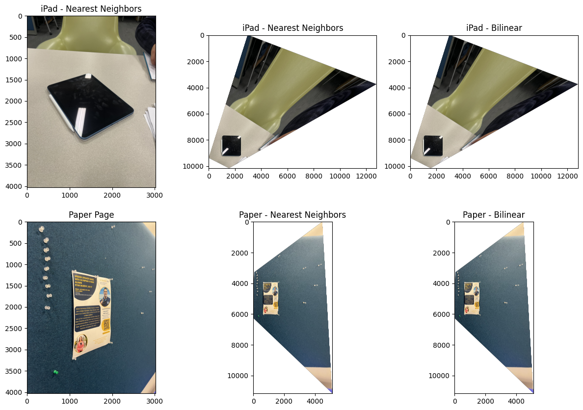
To verify my homography and warping functions were working correctly, I performed rectification on images with rectangular objects (an iPad and a piece of paper). I manually defined correspondences between the rectangles and a standard square, so the homography transformed the distorted objects back to their rectangular shapes.

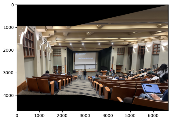
Part A.4: Blend the Images into a Mosaic

Here, I blended the images into a mosaic by warping the images one on top of the other and extending the dimensions accordingly. Also, I added simple feathering at every channel using the alpha channel by setting it to 1 at the center of each image and making it fall off until 0 at the edges.

Blending Procedure

Compute the homography from image 2 to image 1 (src -> dest).
Warp image 2 (and beyond) into image 1 using warpImageBilinear() and include the alpha channel as detailed above (light feathering).
Adjust the bounding box / dimensions / offsets to account for the new image size (find the new min/max x/y values, adjust the offset, expand the height and width of the image).
Blend the images together using the alpha channel values (at each pixel, compute the final color as a weighted average of all contributing images using their alpha masks as weights).

Mosaic Results

Mosaic 1: Landscape Rooftop

Landscape Image 1

Landscape Image 2

Panoramo of Rooftop

Mosaic 2: Landscape Panorama

Library Image 1

Library Image 2

Library Panorama

Mosaic 3: Haas Arch Panorama

Haas Image 1

Haas Image 2

Haas Arch Panoramo

Mosaic 4: Lecture Hall Interior

Lecture Hall Image 1

Lecture Hall Image 2

Panoramo of Lecture Hall (Note: There is some distortion of the men since they were walking during the picture. However, from the text shown on the screen, the warping was accurately done. The men moving adds a time dimension to my image.)

Part B: Feature Matching for Autostitching

Introduction

In Part A, I manually selected point correspondences between images to compute homographies. This process is effective, but quite tedious, time-consuming, and prone to human error. Now, I automated the entire pipeline to detect, describe, and match features between images automatically.

Part B.1: Harris Corner Detection

First, I need to identify the corners in the images. I implemented the Harris Corner Detector to find points that are likely to be good candidates for matching.

Harris Corner Detector Algorithm

Given an image \( I(x,y) \) and window size \( w \), the Harris corner detection algorithm works as follows:

Apply Gaussian blur with \( \sigma_b \), then compute the image derivatives with respect to \( x \) and \( y \), obtaining \( I_x \) and \( I_y \).
Compute the products of derivatives: \( I_{xx} = I_x^2 \), \( I_{yy} = I_y^2 \), \( I_{xy} = I_xI_y \).
For each point \( (u,v) \), define a sliding window \( \mathcal{W} = [u - w/2:u+ w/2, v - w/2:v+w/2] \).
Compute the sums: \( S_{xx} = \sum_{(x,y)\in \mathcal{W}}I_{xx} \), \( S_{yy} = \sum_{(x,y)\in \mathcal{W}}I_{yy} \), \( S_{xy} = \sum_{(x,y)\in \mathcal{W}}I_{xy} \).
Calculate the Harris response: \( h = \frac{S_{xx}S_{yy} - S_{xy}^2}{S_{xx}+S_{yy}} \). This is essentially the determinant over the trace.
Select points where the Harris response exceeds a threshold.

I discarded points within 20 pixels of the image edges to avoid boundary effects as the research paper stated.

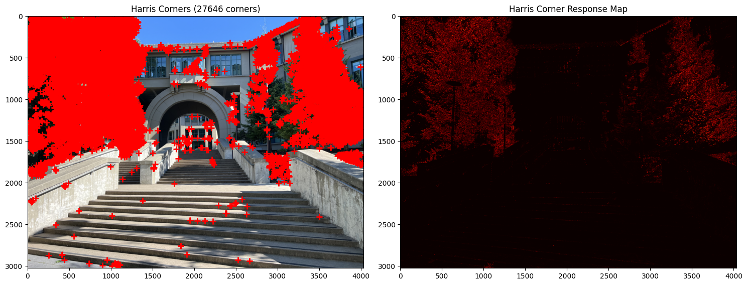
Harris corners detected on the image

Important Note: I added a threshold_rel parameter to the peak_local_max function since running the function without this resulted in over 100,000 points being detected on the image. This led to my kernel crashing in subsequent steps.

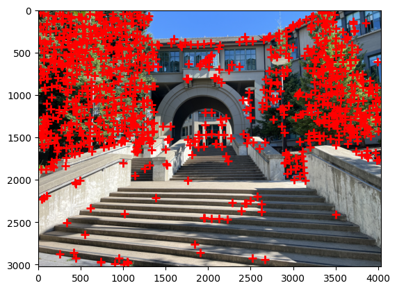
Adaptive Non-Maximal Suppression (ANMS)

To obtain a more evenly distributed set of interest points, I implemented Adaptive Non-Maximal Suppression (ANMS).

ANMS Algorithm

Given Harris corner coordinates coords (N×2) and response values h (N×1), sort corners in descending order by Harris response strength.
For each corner, compute its suppression radius: the minimum distance to a corner with a significantly stronger Harris response (based on the equation f(x) < c * f(y)).
Select the top n corners with the largest suppression radii.

This ensures that selected corners are locally maximal over a large area, promoting even distribution across the image.

After ANMS

Part B.2: Feature Descriptor Extraction

After identifying interest points, I created descriptors that characterize the local appearance around each point. These descriptors allow us to match corresponding points between different images.

Feature Descriptor Pipeline

Extract a 40×40 pixel patch centered at each interest point.
Apply a Gaussian low-pass filter to reduce noise and aliasing.
Downsample the patch to 8×8 pixels (using a spacing of s=5 pixels).
Flatten the 8×8 patch into a 64-dimensional feature vector.
Normalize the descriptor by subtracting its mean and dividing by its standard deviation (bias-gain normalization).

Why 40×40 → 8×8?

The larger 40×40 window captures more context around the interest point. By blurring and downsampling to 8×8, I create a descriptor that is more robust to small variations in position and lighting.

First Image Descriptors

Second Image Descriptors

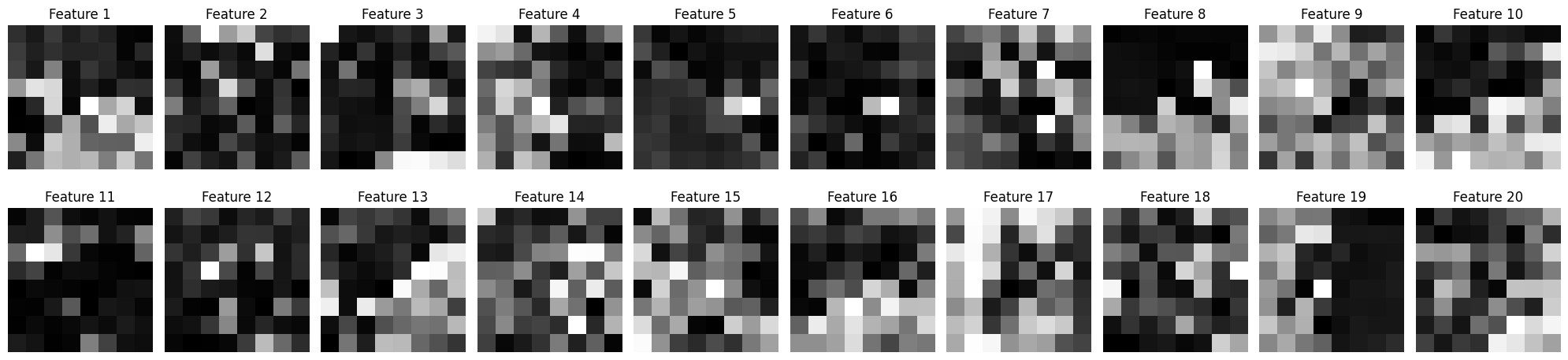
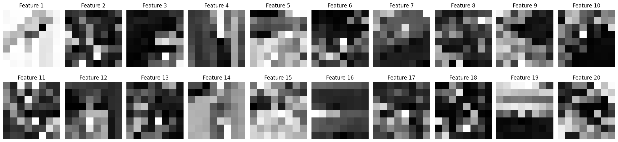
Above: Sample 8x8 patches extracted from interest points

Part B.3: Feature Matching

With feature descriptors computed for both images, I can find correspondences by finding pairs of descriptors that are similar. I implemented a feature matching algorithm that uses the Sum of Squared Differences (SSD) distance metric combined with Lowe's ratio test to identify reliable correspondences.

Feature Matching Algorithm

Compute Pairwise Distances: Calculate the SSD between all descriptor pairs from image 1 and image 2, resulting in an \( n_1 \times n_2 \) distance matrix. I did this using the dist2 function provided by course staff.
For each descriptor in image 1:
- Sort all descriptors in image 2 by their distance to this descriptor.
- Identify the nearest neighbor (NN1) and second-nearest neighbor (NN2).
- Retrieve their distances: \( d_1 \) and \( d_2 \).
Apply Lowe's Ratio Test: Accept the match only if: \[ \sqrt{\frac{d_1}{d_2}} < \text{threshold} \] where the threshold is set to 0.7. This ensures that the best match is significantly better than the second-best match.

Lowe's Ratio Test

The ratio test filters out ambiguous matches. If the nearest neighbor is only slightly closer than the second-nearest neighbor, the match is unreliable. By requiring a significant distance ratio (typically < 0.7), it keeps only high-confidence matches.

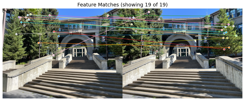
Matched features between two images (different colored lines connect corresponding points)

After feature matching with threshold 0.7, I obtained approximately 20 matches per image pair.

Part B.4: RANSAC for Robust Homography Estimation

Even with careful matching, some outliers (incorrect matches) still exist. RANSAC (Random Sample Consensus) can compute an accurate homography despite the presence of outliers.

4-Point RANSAC Algorithm

Input: Set of matches, number of iterations n_iterations, inlier threshold ε.
Initialize: best_H = None, max_inliers = 0.
Repeat for n_iterations:
- Randomly select 4 point correspondences.
- Compute homography \( H \) from these 4 points (exactly determined system).
- Transform all points from image 1 using \( H \).
- Compute the Euclidean distance between transformed points and their matches in image 2.
- Count inliers: points with distance < ε ( ε = 3 pixels).
- If the number of inliers exceeds max_inliers, update best_H and max_inliers.
Refinement: Recompute \( H \) using all inliers from the best model (least squares).
Output: Final homography best_H.

I used 1000 RANSAC iterations with an inlier threshold of 3 pixels.

Automatic Panorama Stitching Results

Here are comparisons between manually stitched (Part A) and automatically stitched (Part B) panoramas.

Mosaic 1: Library

Manual stitching (Part A)

Automatic stitching (Part B)

Mosaic 2: Haas Building

Manual stitching (Part A)

Automatic stitching (Part B)

Mosaic 3: Outside Landscape

Manual stitching (Part A)

Automatic stitching (Part B)

Analysis and Comparison

The automatic stitching pipeline produces results that are comparable to, and in my opinion for mosaics 1 and 3 better than, manual stitching:

Accuracy: Automatic feature matching identifies correspondences with sub-pixel accuracy, while manual clicking is limited by human precision (most of my correspondences were off by a couple of pixels since I roughly eye-balled them).
Robustness: RANSAC effectively filters out outliers, making the homography estimation more robust to incorrect matches.
Efficiency: The automatic pipeline processes image pairs in a couple of minutes, compared to the time it takes to manually find correspondences per pair of images.
Consistency: Automated methods produce reproducible results, while manual selection introduces variability.

However, automatic methods can struggle in scenarios with repetitive patterns or light changes.