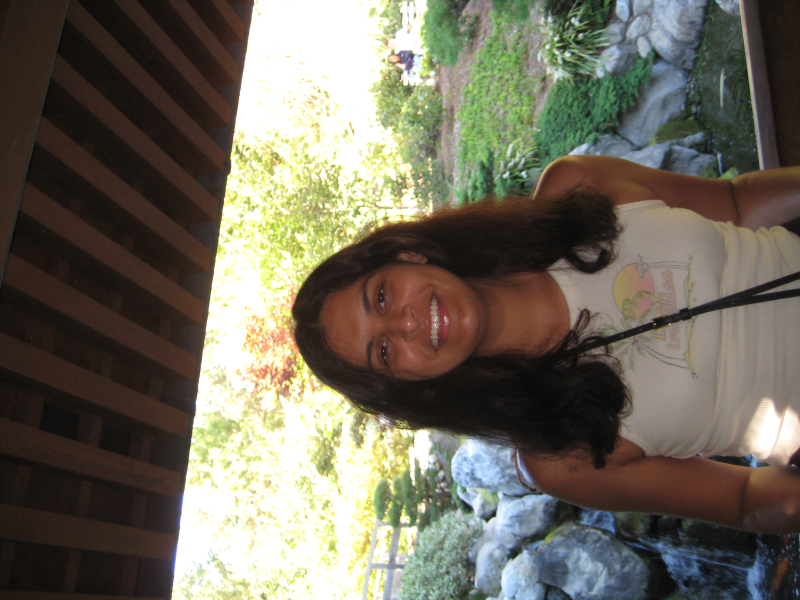
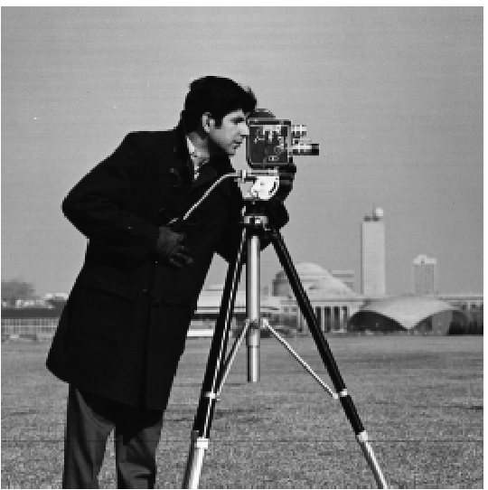
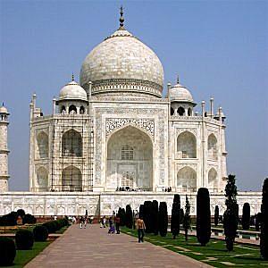
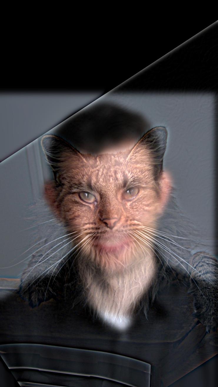
https://aditimundra05.github.io/cs180/3/index.html

Project 2: Filters and Frequencies

Part 1: Filters

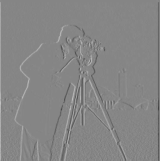
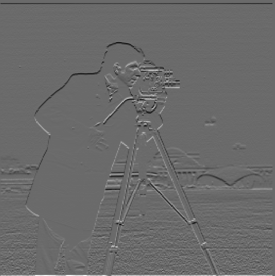
In this part, we'll take x and y partial derivatives of images by convolving them with the finite difference filters Dx and Dy.

Filter Definitions:
Dx = [1, 0, -1] (horizontal finite difference)
Dy = [1; 0; -1]T (vertical finite difference)
G = Gaussian filter with specified σ (sigma)

Part 1.1: Convolutions from Scratch

First, I implemented 2D convolution operations using both four-loop and two-loop approaches with zero-padding support. I compared these implementations against scipy.signal.convolve2d to ensure correctness.

Implementation Approaches:
Four-loop implementation: Nested loops over output height, width, kernel height, and kernel width
Two-loop implementation: Loops over output height and width with vectorized kernel operations
Scipy reference: scipy.signal.convolve2d function
def convolution_four_loops(img, filter): h, w = img.shape fh, fw = filter.shape filter = np.flipud(np.fliplr(filter)) # Flip for convolution output = np.zeros((h, w)) padded = np.zeros((h + 2 * (fh // 2), w + 2 * (fw // 2))) padded[(fh // 2) : (fh // 2) + h, (fw // 2) : (fw // 2) + w] = img for x in range(h): for y in range(w): conv = 0.0 for fx in range(fh): for fy in range(fw): conv += filter[fx, fy] * padded[x + fx, y + fy] output[x, y] = conv return np.clip(output, 0, 1)
def convolution_two_loops(img, filter): h, w = img.shape fh, fw = filter.shape filter = np.flipud(np.fliplr(filter)) # Flip for convolution output = np.zeros((h, w)) padded = np.zeros((h + 2 * (fh // 2), w + 2 * (fw // 2))) padded[(fh // 2) : (fh // 2) + h, (fw // 2) : (fw // 2) + w] = img for x in range(h): for y in range(w): conv = padded[x:x+fh, y:y+fw] output[x, y] = np.sum(conv * filter) return output

Applied a 9×9 box filter to demonstrate equivalence across all three implementations:

Original face image
Original face image
Four loops result
Four-loop convolution result
Two loops result
Two-loop convolution result
Scipy result
Scipy convolution result
Runtime Analysis / Boundary Handling:

The four-loop implementation had the slowest runtime due to the nested loops, while the two-loop implementation had a moderate speedup because the kernel size was indexed instead of being iterated over. However, signal.scipy.convolve2d had the fastest runtime overall since it is optimized C code. All implementations used zero-padding to handle boundaries, specifically mode='same', boundary='fill', fillvalue=0 for the scipy function. The image is padded with zeros by (Kh//2, Kw//2) on all sides, ensuring the output maintains the same dimensions as the input image while properly handling edge pixels.

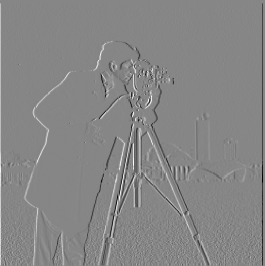
Applied finite difference operators Dx and Dy for edge detection:

Dx face
Dx = [-1, 0, 1] (horizontal edges)
Dy face
Dy = [1; 0; -1]T (vertical edges)

Part 1.2: Finite Difference Operator

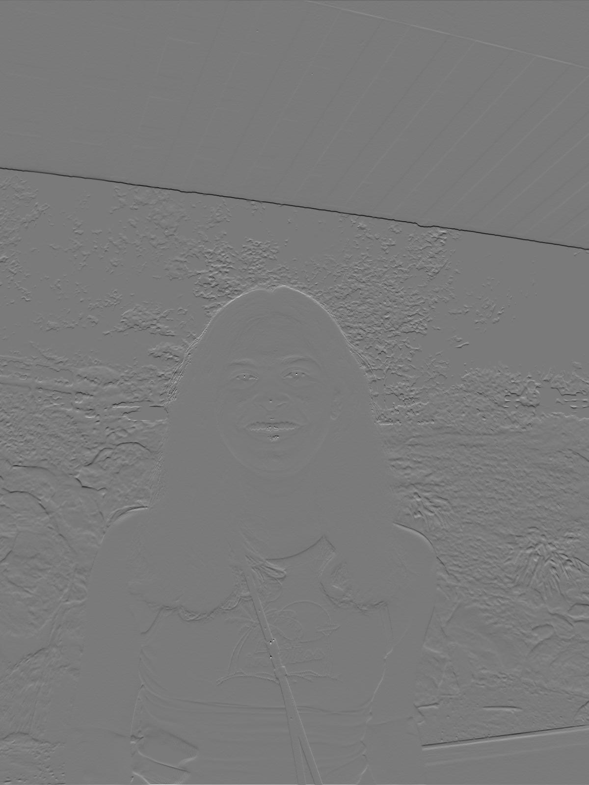
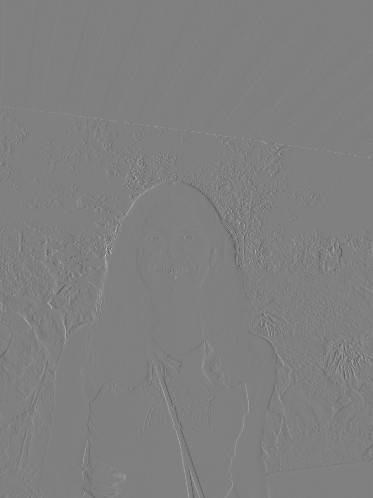
Here, I applied the finite difference operators to the image to demonstrate edge detection capabilities.

Original cameraman
Original cameraman image
Gradient magnitude
Gradient magnitude |∇I|
Dx cameraman
∂I/∂x = I ⊗ Dx
Dy cameraman
∂I/∂y = I ⊗ Dy
Binarized edges
Binarized edges (threshold = 0.35)
Gradient Magnitude Computation:
|∇I| = √((∂I/∂x)² + (∂I/∂y)²)
where ∂I/∂x and ∂I/∂y are computed by convolving I with Dx and Dy respectively.

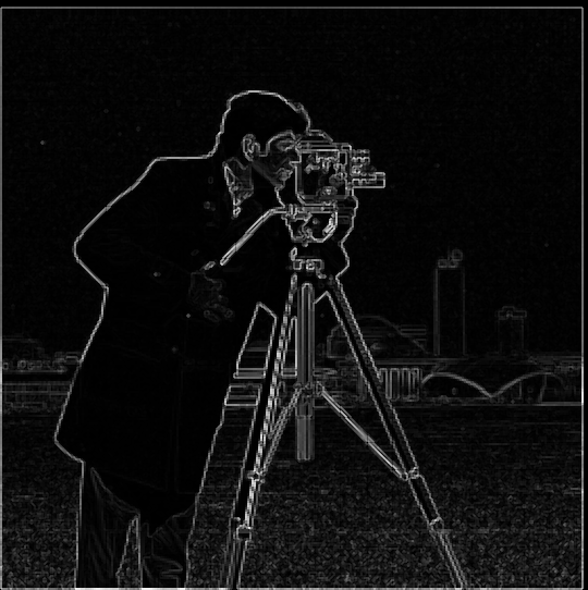
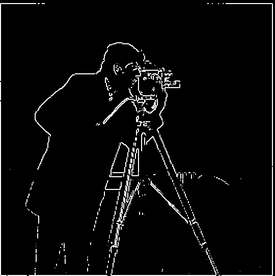
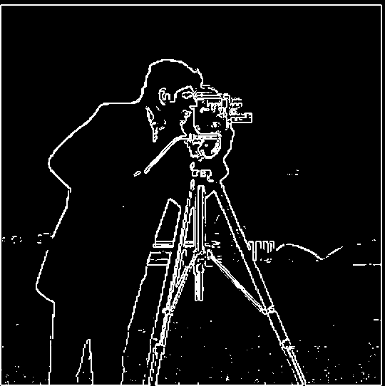
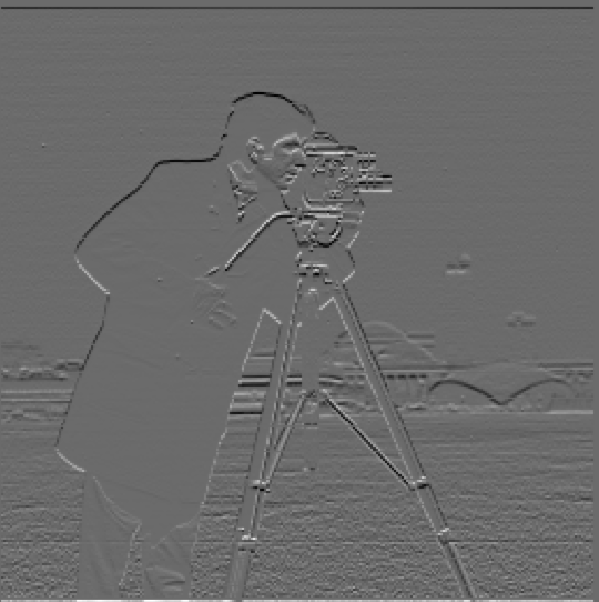
To create an edge detection image, we select a threshold τ and at each position evaluate whether the gradient magnitude is greater than τ. The result is a binary image where pixel value 1 corresponds to the presence of an edge and 0 to the absence of an edge. I tried a couple of thresholds (0.1, 0.2, 0.25, 0.3, 0.4) and 0.35 provided the best balance between finding edges and removing noise. For example, the threshold of 0.2 had more noise (many specs in the background of the grass) and the threshold of 0.4 took away too many edges to properly show the man's figure.

Part 1.3: Derivative of Gaussian (DoG) Filter

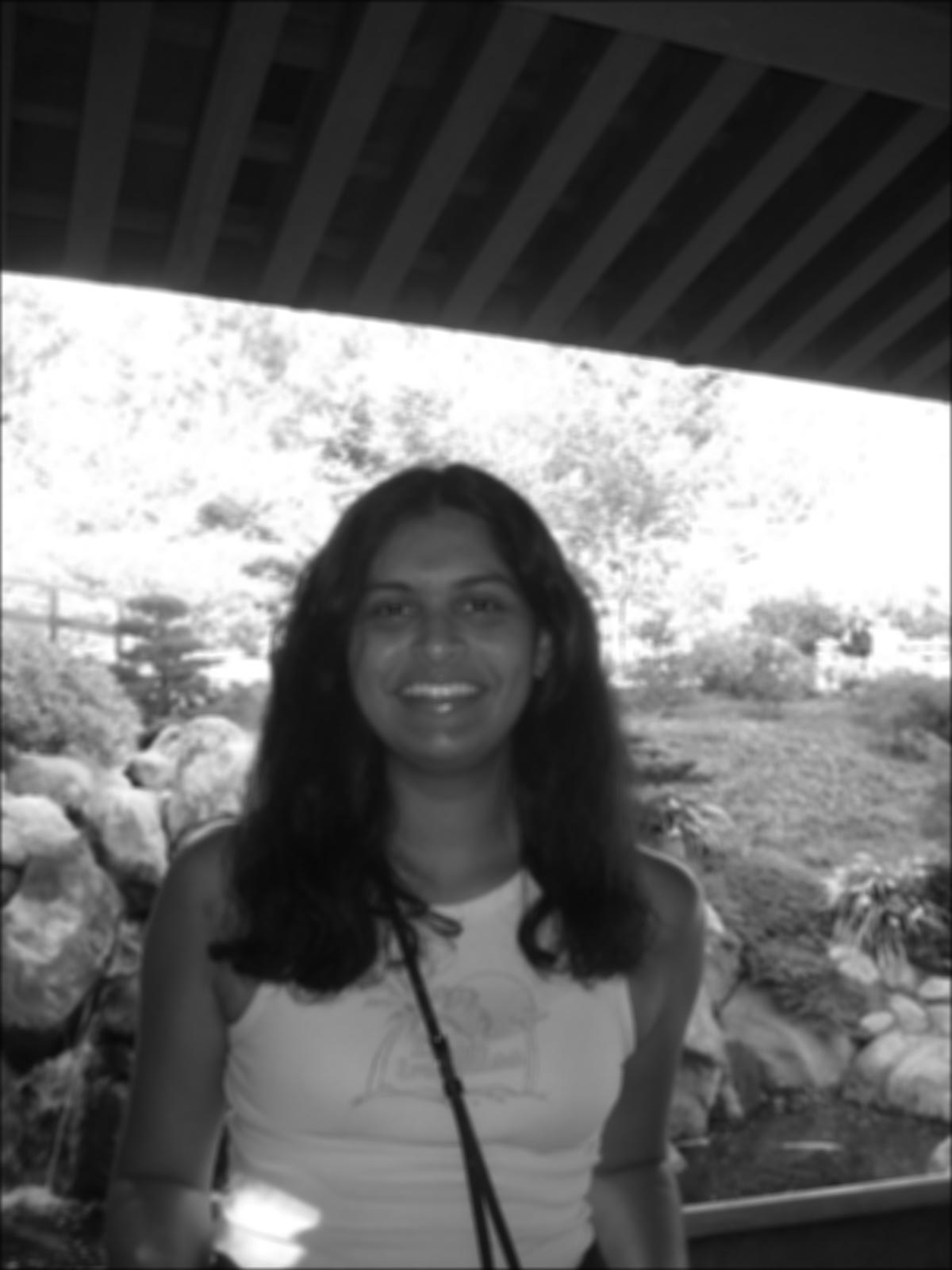
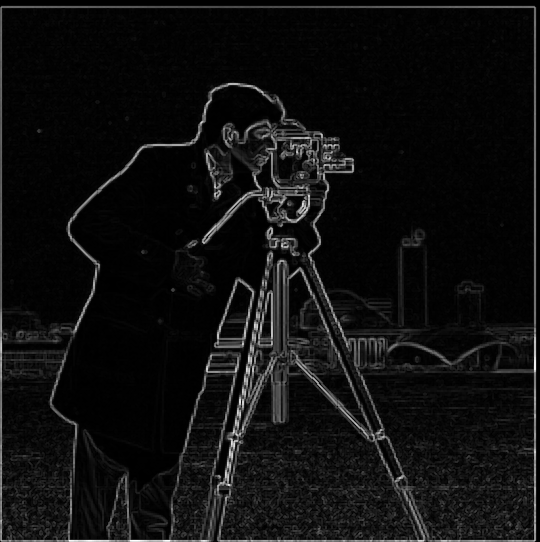
First, I created a gaussian filter using cv2.getGaussianKernel() with a sigma value of 0.5 and n = int(2*np.ceil(3*sigma) + 1). To make it 2D, I took the outer product of this 1D gaussian with its transpose. Then, I convolved the image with the gaussian to smoothen it before taking its x and y partial derivatives like before, getting the gradient magnitude image, and the edge image with a lower threshold than before (0.2 showed the best results). This is compared to the same thing with a single convolution of the gaussian and Dx/Dy (called the derivative of the gaussian), and generating the respective images for comparison.
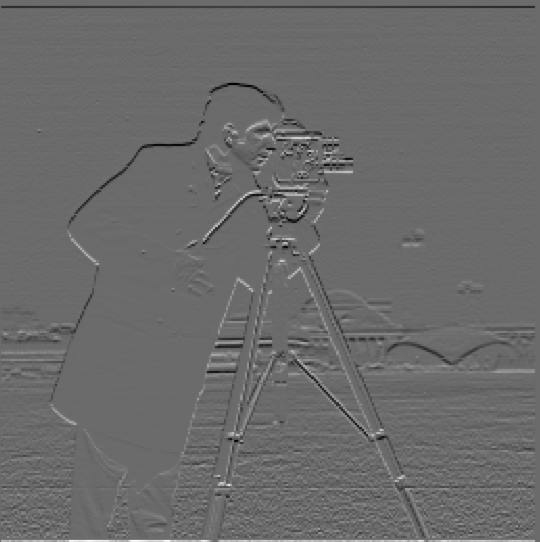
Smoothed gradient magnitude
Smoothed gradient magnitude |∇(G ⊗ I)|
DoG gradient magnitude
DoG gradient magnitude |(DoGx ⊗ I, DoGy ⊗ I)|
Edge smoothed gradient magnitude
|∇(G ⊗ I)| > 0.2
Edge DoG gradient magnitude
|(DoGx ⊗ I, DoGy ⊗ I)| > 0.2
Smoothed dx
∂(G ⊗ I)/∂x
Smoothed dy
∂(G ⊗ I)/∂y

vs.

DoG x result
DoGx ⊗ I
DoG y result
DoGy ⊗ I

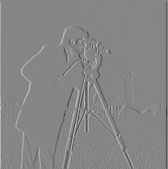
Results are identical due to associativity of convolution!

Gaussian
Gaussian
DoG x
DoGx
DoG y
DoGy
Observations:

Convolution with linear filters is commutative and associative, so convolving I and G, then convolving this with Dx is the same as convolving I with G * Dx. Additionally, compared to the previous section, smoothing the image allows the result to have less white noise and the edges remain preserved.

Part 2: Frequencies

Part 2.1: Image "Sharpening"

Taj Mahal original
Taj (Original, Blurred, High Frequency, and Sharpened)

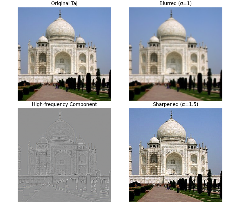
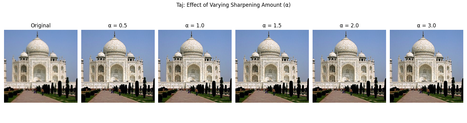
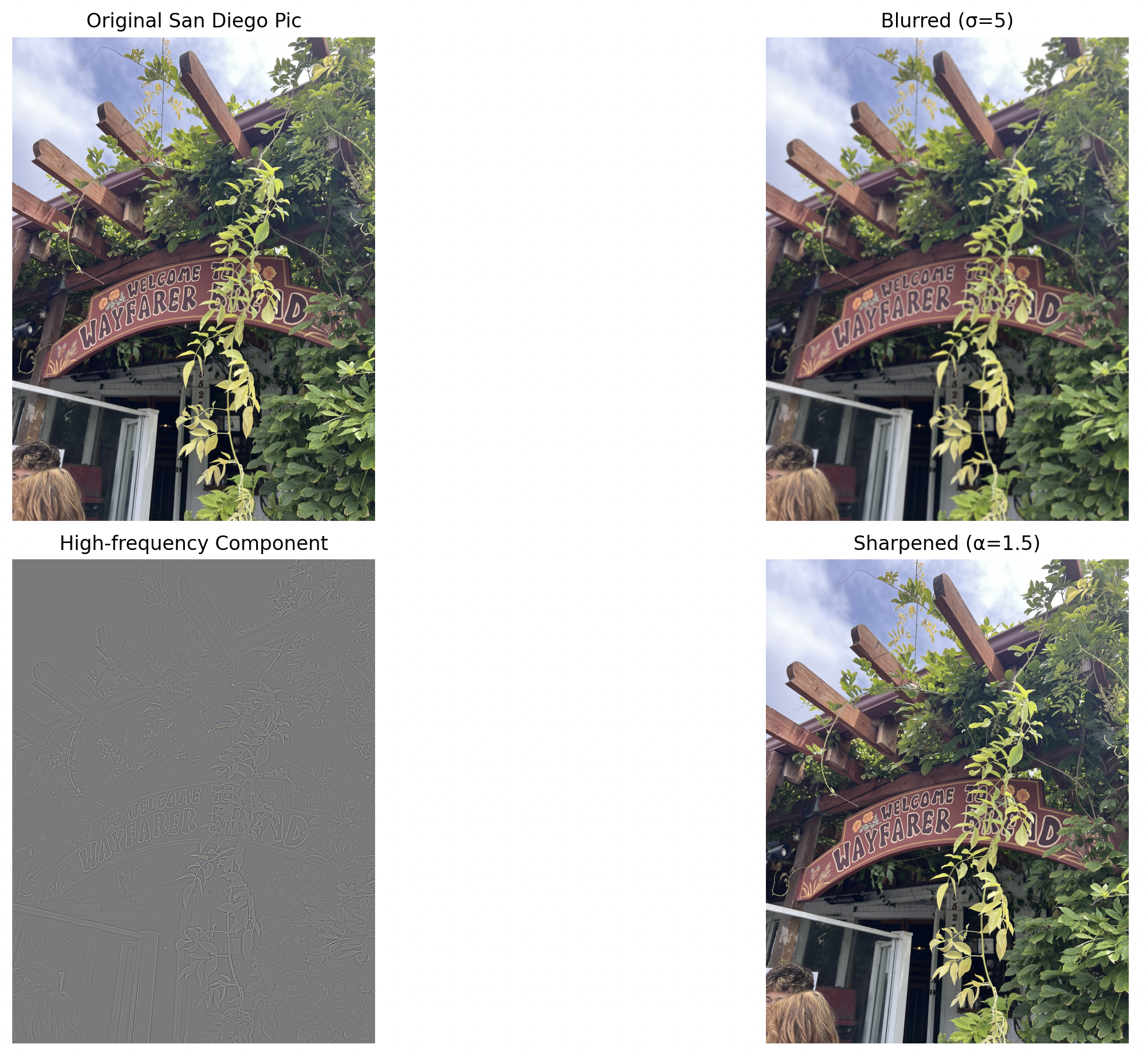
Unsharp masking is a technique that starts off by blurring the original image using a low-pass filter (Gaussian in this case). This blurred image is subtracted from the original image to get the high-frequency components of the image, which correspond to the edges and fine details. Then, this high-frequency information is added back to the original image (by some scaling factor) which increases the edge contrast and makes them appear sharper and more defined. Below, the Taj Mahal is sharpened with varying scaling factors which impacts how pronounced the edges look. Let I denote a given grayscale 2D image, α denote the sharpening parameter, and G denote a gaussian filter.

Unsharp Masking:
sharpened = I + α(I - I ⊗ G)
unsharp_filter = (1 + α)δ - αG
Different Sharpness of Taj
Original Taj
Original Taj Mahal
Sharpened Taj
Sharpened Taj Mahal (α = 1.5)
ZOOM IN TO SEE BETTER: Wayfarer Bakery in SD (Original, Blurred, High Frequency, and Sharpened)

Part 2.2: Hybrid Images

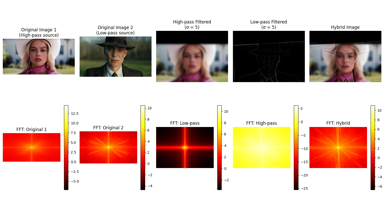
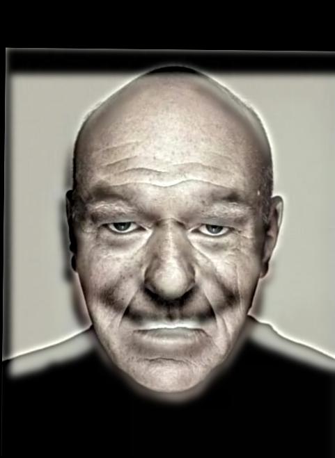
Using the hybrid images approach from the SIGGRAPH 2006 paper, I made static images that change in interpretation as a function of the viewing distance. When viewing these images from a close distance, the high frequency portion of one image is visible and viewing it from afar shows the low frequency portion of the other image.

Hybrid Image Creation Process:
1. Align two input images
2. Apply low-pass filter (Gaussian) to one image: I₁_low = I₁ ⊗ Gσ₁
3. Apply high-pass filter to the other image: I₂_high = I₂ - (I₂ ⊗ Gσ₂)
4. Combine: hybrid = I₁_low + I₂_high
Scary x Smiley Man
Hybrid of Scary x Smiley Man (σ = 5)
Derek x Cat
Hybrid of Derek x Cat (σ = 5)

Part 2.3: Gaussian and Laplacian Stacks

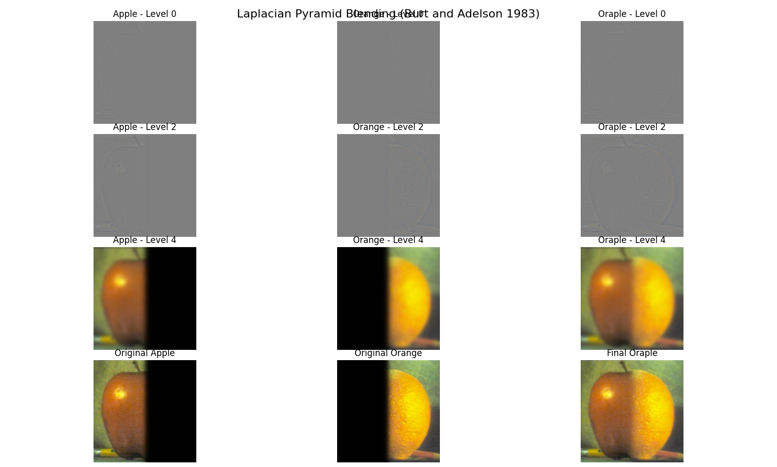
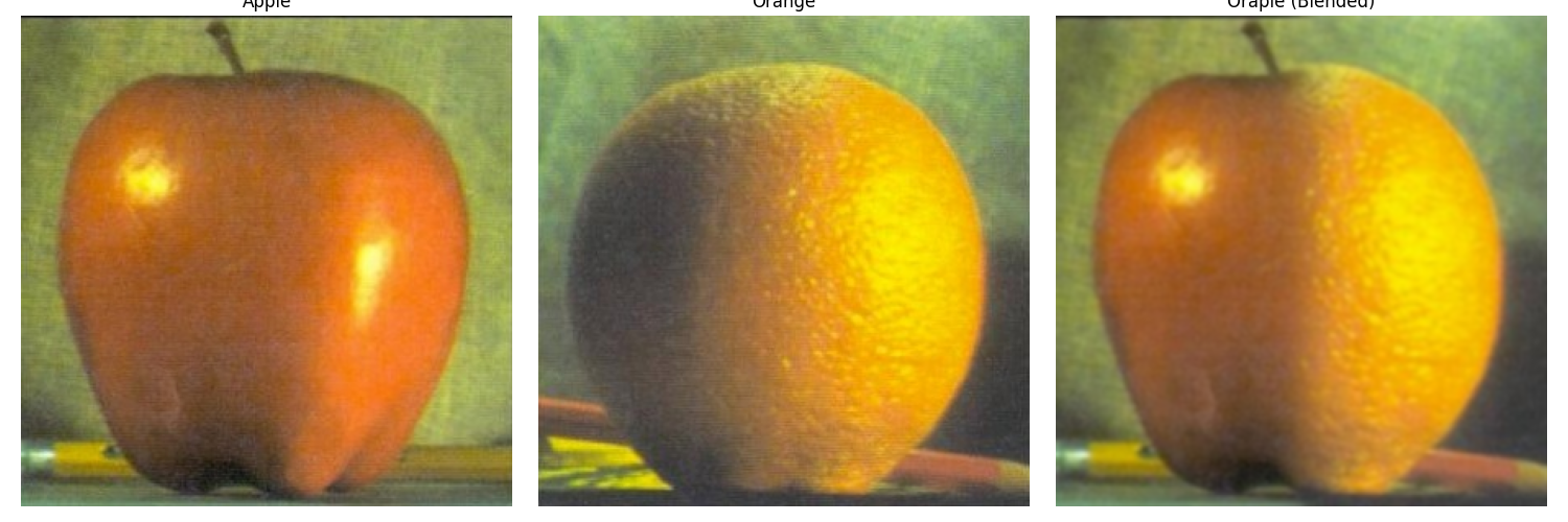
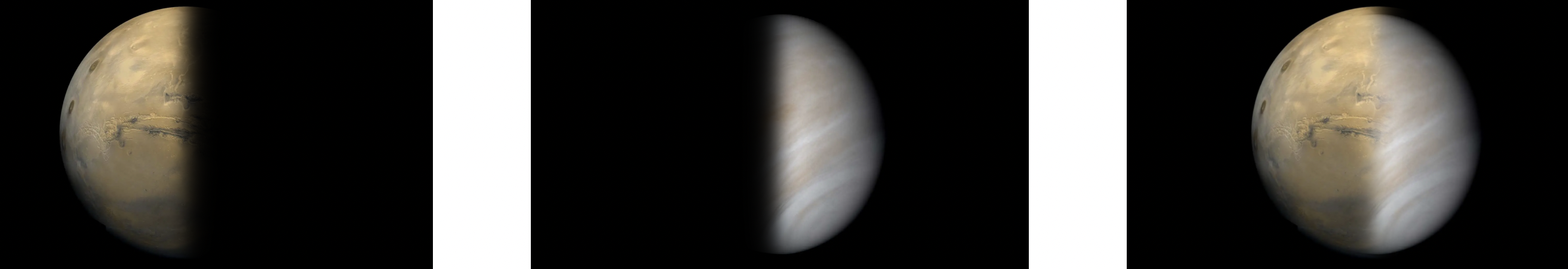
I implemented Gaussian and Laplacian stacks (without downsampling) in preparation for multiresolution blending. Unlike pyramids, stacks maintain the original image dimensions at each level, by applying the Gaussian filter at each level without subsampling.

Masks
Figure 3.42

Part 2.4: Multiresolution Blending

Oraple
Output Oraple Blended
MarsxVenue
Mars x Venus Blended
Earth
Earth
Saturn
Saturn
Earth x Saturn
Smoothed circular mask blend (Earth x Saturn)
Multiresolution Blending Algorithm:
1. Create Gaussian and Laplacian stacks for both input images A and B
2. Create Gaussian stack for the blending mask M
3. For each level k, blend: Lblend[k] = GM[k] ⊙ LA[k] + (1 - GM[k]) ⊙ LB[k]
4. Reconstruct final image: result = Σ Lblend[k]
Multiresolution Blending:
Here, I created blended images of the orange and apple using a smoothed vertical mask along with Mars and Venus. For the irregular mask, I used a smoothed circular mask to blend together Earth and Saturn. In my opinion, the hardest part was finding the right center and radius for the mask to blend the images together since they weren't aligned completely to start off with.